Use of Conditional Formating With COUNTIF Function

Today I am going to share with understanding the Comparison Logic COUNTIF with Conditional Formating, How you can find your Matched and Unmathced data data in two Columns with condition formating.

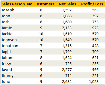
For Example:- Lets assume your data looks like this:

 

In your data range as per above you want to find Duplicate and Unique value and  with conditional formating. If your Select values in first list (assuming the values are in B21:B29).

I have used here Formulas>Define Name  Tab here for giving a Range Name(B21:b29) to lst1.

Same option I have used for giving a Range Name (C21:C28) to lst2.

 Also, you should know how to use COUNTIF Excel Formula

So in order to find-out if a value is in list 1 only, we use a formula like =COUNTIF(lst2,value)=0.

This function will check whether “value” occurs anywhere in lst2 and returns false if that is the case.  (it assumes that value is already in lst1).

Highlighting Items that are in First List Only 

Go to conditional formatting > add rule (Use COUNTIF Function and Set Your Formating as per mentioned Step:-

 Select the rule type as “formula”

 Write a rule like this: =COUNTIF(lst2, B21)=0

 Double check the reference and make sure it is relative (and not like $B$21). Select the reference and press  F4 repeatedly to change it to relative reference.

Set the formatting you want.

It will highlighting Items that are in Second List Only:-

 

 Select values in second list (assuming the values are in C21:C28)

Go to conditional formatting

 Select the rule type as “formula”

 Write a rule like this: =COUNTIF(lst1, C21)=0

 Repeat steps  as  per above. 

Highlighting Values in Both Lists:

Now, it gets interesting as you should apply conditional formatting individually to both lists.

Select values in first list (assuming the values are in B21:B29).

Set the conditional formatting rule as =COUNTIF(lst2,B21)>0

Apply formatting as you want.

Now select second list (assuming the values are in C21:C28)

Set the conditional formatting rule as =COUNTIF(lst1,C21)>0

Again, apply formatting as you want.

Hope you learned something out of this trick.  "HAPPY LEARNING"

Use of vlookup With-wild-card-example

Dear All,

For Example. In the below data, we may not remember the full name of sales person, but we know that her/his name starts with jac. Now how do you get the sales amount for that person?

Data:

Solution

Simple. Use wild cards. Like this: =VLOOKUP("jac*",$B$5:$E$17,3,FALSE) to fetch the value from 3rd column for the person whose name starts with jac

Examples:

Hope you learned something out of this trick.  "HAPPY LEARNING"